

Summary
This study seeks to present an approach for designing machine-learning control applications, to achieve critically-damped responses in single-degree-of-freedom systems, that can be applied to more complex multi-degree-of-freedom systems. The investigation is motivated by the usefulness that this type of conclusion would provide for controlling dynamic systems where closed-form solutions achieved with analytical methods do not exist.
The potential solutions are proposed:
- Building a Random Forest Regressor
- Building a Collaborative Filtering Regressor
Both are evaluated qualitatively and quantitatively by first discussing the advantages and disadvantages of both from the literature [1]; and then training, evaluating, interpreting, adapting, and re-evaluating both models.
After one iteration of quantitative evaluation, random forest regression is put forward as the more viable of the two, achieving a root-mean-squared error of 47.7012, as opposed to 149.0302 for collaborative filtering regression. The associated design approach is to,
- collate an expansive and accurate dataset using transfer-function analysis and the principle of superposition,
- build a random forest model, and
- use the random forest to recursively interpret, adapt, and re-evaluate the dataset and random forest models.
While neither model is particularly good at predicting the input required to achieve a critically damped response for the system used to generate the dataset nor are they suitable for applications in higher-degree-of-freedom systems, the conclusion presented in this report serves as a foundation upon which to conduct further investigation and design approach development.
1. Background
Frequency-domain transfer functions are commonly used in automatic control engineering to analyze, model, and control dynamic systems. Extensive study of Laplace transform and dynamic/electric-circuit system theory has resulted in well-established analytical solutions to common systems. Typically, the ordinary differential equations describing these dynamic and electric circuit systems are converted to the frequency domain a Laplace transform, where they are more easily studied, before reverse Laplace transforming results back to the more-easily-interpreted time domain. Challenges arise when systems deviate from classical archetypes, for which well-established analytical solutions exist, or when multiple degrees of freedom become involved. Methods exist to address these situations, but are often computationally rigorous and yield results that may not be reliable.
Machine learning is an engineering tool whose evolution into mainstream usefulness far succeeds the aforementioned traditional automatic control engineering methods. However, machine learning’s advantages may be relevant to or even resolve some of the more prominent issues of automatic control engineering.
One specific case in which computational or high-degree-of-freedom challenges may be resolved by machine learning control applications is achieving a critically damped response in dynamic and eclectic circuit systems. This type of response is desirable whenever system outputs are changed from one level to another. It provides fast convergence when big changes are needed but exponentially slows its approach to avoid overshoot.
This report seeks more clarity on the applicability of modern machine-learning approaches to dynamic/electrical circuit system control for this exact scenario—critically damped response for output parameter changes.
2. Introduction and Scope
Here, the scope of this study is defined explicitly by making a problem and objective statement and discussing some goals and limitations involved with the methods used.
2.1 Problem
Designing control applications to produce critically damped dynamic system responses is difficult when characteristic transfer functions are not immediately evident.
2.2 Objective
The objective of this report is to
provide a general approach to machine learning-based control application design for critically damped single-degree-of-system system responses that can be extrapolated to multi-degree-of-freedom systems.
2.3 Goals
To expand on the objective, several specific goals for this study are defined. The machine-learning control application design approach put forward in the conclusion as the best, over the alternatives studied, must
- control a single-degree-of-freedom dynamic system to have a critically-damped response, and
- show promise, with further testing, to be equally as applicable in higher-degree-of-freedom systems.
A successful conclusion of this study will present
- a choice of one potential solution as the “best” over the alternatives,
- a quantitive warrant for this distinction, and
- a qualitative discussion of the “best” potential solution’s usefulness for higher-degree-of-freedom systems.
2.4 Methods
An evaluative analysis method is used to achieve the objective of this study:
- Several potential solutions are introduced.
- An initial, qualitative assessment is made based on information provided in the literature [1].
- A secondary, quantitative assessment is made by testing the accuracy of each potential solution with the same training and validation datasets.
- One potential solution is put forward as the quantitative and qualitative “best” and its ability to better meet the objective over the alternative potential solutions is discussed.
2.5 Limitations
The finite scope of this report limits the conclusion that can be drawn. The accuracy that the solution, proposed in this report, achieves for a single-degree-of-freedom dataset will be stated explicitly; however, no actual testing will be done for multi-degree-of-freedom datasets. Instead, only a qualitative discussion of its usefulness in these settings will be included. Before the proposed machine-learning control application design solution is used for higher-order systems, rigorous testing for this type of use case should be done.
3. Potential Solutions
Design approaches for two machine learning architectures, suitable for the current control problem, are proposed in this section:
- Random Forest Regression
- Collaborative Filtering Regression
Machine learning is the process of building an architecture and training it into a model to accurately map a set of independent variables to a dependent one. A diverse range of architectures exists, ranging from decision trees that build a predictable structure with a known algorithm to neural networks which adapt their structure unpredictably with stochastic gradient descent.
3.1 Potential Solution I: Random Forest Regression
Like decision trees, random forests use an algorithm to structure a series of independent-data splitting criteria so that they can organize data into groupings that accurately predict the dependent variable. [1] Random forests differ by building multiple decision trees with subsets of the training dataset and using the aggregate of those trees’ predictions—a method proposed and analyzed by Breiman in Bagging PredictorsI [2].
Refer to pages 287–314 of the literature [1] for a detailed explanation of this regression method.
The random forest architecture is implemented in Google Colab by defining a function which calls the `RandomForestRegressor` function [3] from the `sklearn` library [3]:
def rf(xs, y, n_estimators = 40, max_samples = 200, max_features = 0.5, min_samples_leaf = 5, **kwargs):

  return RandomForestRegressor(n_jobs = -1, n_estimators=n_estimators, max_samples=max_samples, max_features=max_features, min_samples_leaf=min_samples_leaf, oob_score=True).fit(xs, y)
Each of the following parameters passed to `RandomForestRegressor` plays an influential role in the construction and performance of the random forest:
- `n_estimators` defines the number of trees wanted,
- `max_samples` defines the number of rows to sample in each training tree,
- `max_features` defines how many columns to sample at each split point,
- `min_samples_leaf` defines the minimum number of samples that a leaf node can split off, and
- `n_jobs = -1` specifies that all trees should be built in parallel using all CPUs. [1]
3.2 Potential Solution II: Collaborative Filtering Regression
Collaborative filtering is an architecture that uses neural networks to learn latent-value vectors for each row and column in a dataset so that their dot products accurately predict the data in the associated row/column intersection. [1]
Refer to pages 253–276 and 314–328 of the literature [1] for a detailed explanation of this regression method.
The collaborative filtering architecture is implemented in Google Colab as a `tabular_learner` object [3] from `fastai.tabular.data` library [4]:
learn = tabular_learner(dls, y_range = (-75, 180), layers = [500,250], n_out = 1, loss_func = F.mse_loss)
The `tabular_learner` object is passed the following parameters which influence the neural network assigned and the way it is trained:
- `dls` is the `dataloaders` passed to the `tabular_learner` (defines how data is passed to the model)
- `y_range` defines the upper and lower bounds for regression
- `layers` defines the number of activations for the first and second layers of the neural network,
- `n_out` defines the number of outputs, and
- `loss_func` specifies which loss function should be used. [1]
4. Initial Assessment
An initial assessment of potential solutions is done qualitatively by reviewing the advantages and disadvantages put forward in the literature and discussing them here.
4.1 Case Study
The differences between collaborative filtering and random tree regression are well-illustrated by a case study in the literature [1] (on page 314). Howard and Gugger [1] use a random forest to try and predict the linear relationship of 40 “slightly noisy” data points. The results reveal that the random forest architecture is unable to extrapolate outside the domain of the training data. Howard and Gugger [1] explain that this limitation extends beyond time-domain data to more general cases as well.
Without any further intervention, the random forest model has a root-mean-squared error rate of 23.3% for this reason. [1] By removing redundant data (columns that are not useful as well as old data) the model is made simpler and more resilient, and the error is decreased marginally to 23.0%. [1] However, only with the addition of neural networks can the root-mean-squared error rate be reduced to 22.2% (which corresponds with an accuracy of 94.9%). [1]
Through this example, Howard and Gugger [1] point out the tradeoff between the superior ability of collaborative filtering models to extrapolate, and the superior ability of random forest models to provide reliability within the domain of their training data. This compromise is summarized in the following subsections:
4.2 Random Forest Regression
Likewise, the following advantages and disadvantages of Random Forest regression can be inferred from Howard and Gugger’s [1] discussion of the architecture:
Table 1: Qualitative Advantages and Limitations of Random Forest Regression
| Advantages | Limitations |
|
|
4.3 Collaborative Filtering Regression
The following advantages and disadvantages of Collaborative Filtering regression can be inferred from Howard and Gugger’s [1] discussion of the architecture:
Table 2: Qualitative Advantages and Limitations of Collaborative Filtering Regression
| Advantages | Limitations |
|
|
Interpreting the advantages and limitations outlined above reveals some important qualitative distinctions between Potential Solution I and Potential Solution II:
Potential Solution I. uses random forest regression and can be generalized to have reliable performance in interpolation, but a poor ability to extrapolate to data not seen in training; whereas Potential Solution II., which uses collaborative filtering regression, can be generalized to have good performance in extrapolation.
5. Engineering Analysis
The engineering analysis for this study is performed by
- Collating a dataset.
- Assigning a metric for comparison and evaluation.
- Separating the dataset into training and validation subsets.
- Building, and evaluating a Random Forest Regressor (Potential Solution I).
- Building, training, and evaluating a Collaborative Filtering Regressor (Potential Solution II).
- Interpreting, adapting, and re-evaluating the design methods.
Steps 2 through 6 of this analysis procedure closely follow the procedure outlined in “Chapter 9” of Howard and Gugger [1].
5.1 Dataset
Appropriate data is critical to the validity and applicability of this study. A dataset that mimics the intended application of the ML control application design approach, proposed in the conclusion of this report, is used so that the method’s performance in a relevant situation can be assessed directly.
A custom dataset is constructed by considering a situation for which a known analytical solution exists. The image below is the transfer-function-representation of a single-degree-of-freedom system that takes an input, $R\left(s\right)$, to achieve a critically damped response, $Y\left(s\right)$, while experiencing some interfering disturbance, $D\left(s\right)$, and noise, $N\left(s\right)$.

Figure 1: Transfer-Function Representation of 1DoF System
For the sake of simplicity, the interfering disturbance, $D\left(s\right)$, and noise,$N\left(s\right)$, are considered to be harmonic. Consider the following signals in their time- and frequency-domain representations:
Table 3: Time- and Frequency-Domain Signals
| Signal | Time-Domain Representation | Frequency-Domain Representation |
| Response | $y\left(t\right) = \text{sp}_{i-1} + \left(\text{sp}_{i} – \text{sp}_{i-1}\right) \left(1-e^{-2\pi t}\right)$ | $Y\left(s\right) = \dfrac{\text{sp}_{i-1}}{s} + \left(\text{sp}_{i} – \text{sp}_{i-1}\right) \left(\dfrac{2 \pi}{s\left(s+2\pi \right)}\right)$ |
| Disturbance | $d\left(t\right) = \left(4\right)\cos\left(\dfrac{\pi}{5}t\right)$ | $D\left(s\right) = \left(4\right) \left(\dfrac{\left(\dfrac{\pi}{5}\right)}{s^2 + \left(\dfrac{\pi}{5}\right)^2}\right)$ |
| Noise | $n\left(t\right) = \left(0.5\right)\cos\left(4\pi t\right)$ | $N\left(s\right) = \left(0.5\right) \left(\dfrac{s}{s^2 + \left(4\pi \right)^2}\right)$ |
| Input | Unknown | Unknown |
The linearity of the differential equations defining the behaviour of this system permits the use of superposition in its analysis. So, the response can be written as the sum of the response due to each of the input signals (input, disturbance, and noise):
$$Y\left(s\right) = Y_{R}\left(s\right) + Y_{D}\left(s\right) + Y_{N}\left(s\right)$$
$$Y\left(s\right) = G_{R}\left(s\right) R\left(s\right) + G_{D}\left(s\right) D\left(s\right) + G_{N}\left(s\right) N\left(s\right)$$
$$\dfrac{\text{sp}_{i-1}}{s} + \left(\text{sp}_{i} – \text{sp}_{i-1}\right) \left(\dfrac{2 \pi}{s\left(s+2\pi \right)}\right) = \left(\dfrac{1}{\left(s+2\right)\left(s+3\right)+1}\right) R\left(s\right) + \left(\dfrac{1}{\left(s+2\right)\left(s+3\right)+1}\right) \left(\left(4\right) \left(\dfrac{\left(\dfrac{\pi}{5}\right)}{s^2 + \left(\dfrac{\pi}{5}\right)^2}\right)\right) + \left(-\dfrac{1}{\left(s+2\right)\left(s+3\right)-1}\right) \left(\left(0.5\right) \left(\dfrac{s}{s^2 + \left(4\pi \right)^2}\right)\right)$$
Rearranging, the frequency-domain input, $R\left(s\right)$, can be found:
$$R\left(s\right) = \left(\left(s+2\right)\left(s+3\right)+1\right) \left[ \left( \dfrac{\text{sp}_{i-1}}{s} + \left(\text{sp}_{i} – \text{sp}_{i-1}\right)\right) \left(\dfrac{2 \pi}{s\left(s+2\pi \right)}\right) – \left(\dfrac{1}{\left(s+2\right)\left(s+3\right)+1}\right) \left(4\right) \left(\dfrac{\left(\dfrac{\pi}{5}\right)}{s^2 + \left(\dfrac{\pi}{5}\right)^2}\right) + \left(-\dfrac{1}{\left(s+2\right)\left(s+3\right)-1}\right) \left(0.5\right) \left(\dfrac{s}{s^2 + \left(4\pi \right)^2}\right) \right] $$
Tanking the Inverse Laplace Transform, the time-domain input can be found:
$$\mathscr{L}^{-1}\left\lbrace R\left(s\right) \right\rbrace $$
Note: Taking the Inverse Laplace Transform of this expression is very complex and results in an equation of many terms. For this reason, Wolfram Alpha, an online math solver, was used to obtain the following expression:
a ≡ $\text{sp}_{i-1}$; b ≡ $\text{sp}_{i}$
= (cos(4 π t) 125.7 seconds + sin(4 π t) -2053 seconds + sin(4 π t) -24937 seconds + sin(4 π t) -35 seconds)/(8 π (25 + 240 π^2 + 256 π^4)) + (-15 e^((-5/2 - sqrt(5)/2) t) + 5 sqrt(5) e^((-5/2 - sqrt(5)/2) t) + 15 e^((sqrt(5)/2 - 5/2) t) + 5 sqrt(5) e^((sqrt(5)/2 - 5/2) t) - 32 π^2 e^((-5/2 - sqrt(5)/2) t) + 32 π^2 e^((sqrt(5)/2 - 5/2) t)) -8.182×10^-6 seconds - 2 π (a - b) δ(t) + (e^(-2 π t) (8 π^3 a - 16 π^2 a + 4 π a + 7 a - 8 π^3 b + 20 π^2 b - 14 π b))/(2 π) + (-4 π a - 7 a + 14 π b)/(2 π) + 7 a t - 4 sin((π t)/5)
Implementing this in Google Sheets, where the complete dataset is generated, the complex number term(s) are excluded and the Dirac Delta function is approximated to zero because no zero times exist in this numeric dataset.
Represented graphically, the time-domain data can be seen in the following image:
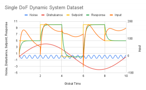
Figure 2: Time-Domain Dataset
Represented tabularly, the first five rows (of 5000) of time-domain data can be seen in the following table:
Table 4: First Five Rows of Tabulated Dataset
| time | time _shifted | setpoint | setpoint _previous | disturbance | disturbance _gradient | noise | noise _gradient | response | response _gradient | input | |
| 0 | 0.002 | 0.002 | 5 | 0 | 0.0050 | 2.5133 | 0.4998 | -0.2368 | 0.0624 | 30.8295 | -15.6948 |
| 1 | 0.004 | 0.004 | 5 | 0 | 0.0101 | 2.5133 | 0.4994 | -0.2368 | 0.1241 | 30.8295 | -13.4245 |
| 2 | 0.006 | 0.006 | 5 | 0 | 0.0151 | 2.5133 | 0.4986 | -0.3945 | 0.1850 | 30.4445 | -11.17961 |
| 3 | 0.008 | 0.008 | 5 | 0 | 0.0201 | 2.5132 | 0.4975 | -0.5520 | 0.2451 | 30.0643 | -8.9600 |
| 4 | 0.01 | 0.01 | 5 | 0 | 0.0251 | 2.5132 | 0.4961 | -0.7091 | 0.3045 | 29.6889 | -6.7653 |
Here numerical gradients have been added for each of the signals with the following formula:
$$\dfrac{d}{dt}\left[s\left(t\right)\right]_{i} = \dfrac{s\left(t_{i}\right)-s\left(t_{i-1}\right)}{t_{i}-t_{i-1}}$$
5.2 Qualitative Evaluation
The error of each model is reported as root-mean-squared error (RMSE):
$$\text{RMSE} = \sqrt{\dfrac{\sum_{i = 1}^{N}\left(x_{i}-\hat{x}_{i}\right)^2}{N}}$$
In the Google Colab integrated development environment (IDE), this is implemented as a function that uses multiple methods from Python’s math library: [1]
def r_mse(pred, y): return round(math.sqrt(((pred-y)**2).mean()), 6)
def m_rmse(m, xs, y): return r_mse(m.predict(xs), y)
5.3 Training and Validation Subsets
The complete dataset of 5000 independent data points is separated into training and validation subsets. The training set is used to train the collaborative filtering model and build the random tree model, while the validation set is held aside so that both models can be validated with data they have never seen before.
Since the control application is intended for projecting into the future, the validation set is selected to succeed the training set.
In Google Colab this separation of data is implemented by assigning the split condition as 8.002 seconds, following Howard and Gugger’s [1] method:
cond = (df.time < 8.002)
train_idx = np.where( cond)[0]
valid_idx = np.where(~cond)[0]

splits = (list(train_idx), list(valid_idx))
Since the dataset covers 10.000 seconds total, this assigns the first 80% of the dataset to training and the latter 20% to validation.
5.4 Random Forest Regressor
An instance of the RandomForestRegressor class with parameters defined in §3.1 is created for the relevant dataset is created by calling the rf function:
m = rf(xs,y)
After building this random forest model with 40 separate trees that each separate the data down to groupings of 25 or more, the RMSE of the model’s predictions for the training and validation datasets are printed:
m_rmse(m, xs, y), m_rmse(m, valid_xs, valid_y)
>> (7.442496, 47.701194)
5.5 Collaborative Filtering Regressor
The collaborative filtering regressor, proposed in §3.2, is trained for five epochs using the .fit_one_cycle method [4] from the fastai library [4]:
learn.fit_one_cycle(5,6918e-3)
The learning rate (the second parameter passed into .fit_one_cycle) for training is selected using Leslie Smith’s .lr_find utility from the fastai library [4]:
learn.lr_find()
>> SuggestedLRs(valley=0.0006918309954926372)
After this five-epoch training period the RMSE of the model’s predictions for the latter 20% of the dataset is printed:
preds, targs = learn.get_preds()
r_mse(preds,targs)

>> 171.171292
5.6 Interpretation, Adaptation, & Re-evaluation
Fundamentally, decision tree models tend to be easier to interpret than collaborative filtering models. The algorithm for building a decision tree is defined and each step that the computer performs and how the data is interacted with is well understood. [1] However, for neural networks, which constitute the learning part of collaborative filtering, the exact way that the model interacts with the data is less well understood. [1]
Accordingly, the random forest fitted to the dataset is interpreted and any helpful conclusions are implemented for both the collaborative filtering regressor and the random forest regressor. Among the methods of interpretation are,
- feature importance, and
- similar features.
The information gathered from these points of interpretation can be leveraged by
- removing low-importance variables, and
- removing redundant variables.
Feature Importance
Feature importance can be studied by parsing through a decision tree to determine for which independent data (columns) splitting criteria results in the greatest reduction of the model’s prediction error. [1]
Howard and Gugger [1] implement this in Google Colab by defining and calling a function called `rf_feature_importance` whose returned data can then be plotted with `matplotlib.pyplot` library [5] functions:
def rf_feat_importance(m, df):
  return pd.DataFrame({'cols':df.columns, 'imp':m.feature_importances_}).sort_values('imp', ascending=False)
fi = rf_feat_importance(m, xs_tindep)
fi[:10]
from matplotlib.pyplot import legend
from IPython.core.pylabtools import figsize
def plot_fi(fi):
  return fi.plot('cols', 'imp', 'barh', figsize=(12,7), legend=False)

plot_fi(fi[:30]);
For the current decision tree, the following plot is printed:

Figure 3: Feature Importance
Column data with short bars represent data that is not particularly influential in the random forest, and that could be removed with little impact on the overall model. [1] In this case, `setpoint` and `noise_gradient` are removed. (See page 305 of the literature [1] for the implementation.)
When this is done, the validation RMSE of the decision tree increases from 47.7012 to 51.5970; however, the model is simpler with only eight columnated entries for each datapoint instead of 10.
Feature Similartiy
Feature similarity can be studied by plotting the feature importance data generated above in a way that indicates when two similar pieces of column data are separated in each decision tree in order of importance. In Google Colab, this can be implemented with a cluster plot: [1]
cluster_columns(xs_imp)
For the current random forest, the following plot is printed:
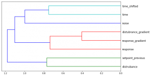
Figure 4: Feature Similarity
Column data linked near the right is split later on and the splitting criteria have less influence on the prediction than splits that occur further to the left. [1] Since `disturbance_gradient` and `response_gradient` appear to be similar, the out-of-bag score of the random forest when each is removed in turn is compared to a baseline when neither is removed: [1]
Baseline:
get_oob(xs_imp)
>> 0.9960
When `disturbance_gradient` and `response_gradient` are removed in turn:
{c:get_oob(xs_imp.drop(c, axis=1)) for c in ('distubrance_gradient', 'response_gradient')}

>> {'distubrance_gradient': 0.9957,
 'response_gradient': 0.9920}
Out-of-bag score is a value generated by `sklearn` [4] that is 1.0 for a perfect model and 0.0 for a random model. (See page 306 of the literature [1] for a detailed description.)
Since neither out-of-bag scores are better than the baseline when both are removed neither parameter is removed. (See pages 307–308 of the literature [1] for a detailed description of out-of-bag scores.)
6. Discussion
The results of the engineering analysis performed on the two proposed machine learning control application design methods are best summarized in a table:
Table 5: Machine Learning Control Application RMSEs
| Random Forest Regression | Collabove Filtering Regression | ||
| Pre- “Interpretation, Adaptation, & Re-evaluation” | Training RMSE | 7.4425 | N/A |
| Validation RMSE | 47.7012 | 171.1713 | |
| Post- “Interpretation, Adaptation, & Re-evaluation” | Training RMSE | 9.9961 | N/A |
| Validation RMSE | 51.1485 | 149.0302 | |
The validation RMSE is the relevant parameter because it indicates how well the random forest regression and collaborative filtering regression models perform on data they have not seen before.
Both are relatively high, indicating that neither control application is particularly good at achieving a critically-damped response for the dataset used in this study. However, the validation RMSEs indicate that the random forest regressor has a substantially lower RMSE than the collaborative filtering regressor.
The relatively high error rates of both models could be indicative of two events:
- Limitations of the dataset, including quantity (not enough) or inaccuracy.
- The unsuitability of the proposed machine learning models to the problem being solved.
While both are possible, the former is discussed in more detail because it should be disproven before concluding the latter. Figure 2 shows the dataset plotted across the time domain. Inspection of this image reveals that the dataset includes only five examples of critically damped responses and one unique cycle of the harmonic disturbance function. Moreover, the dataset includes only 5000 data points. This is to say that the performance of both models could be improved with a more expansive dataset that represents more possible permutations of response, disturbance, noise, and input with more data points. With the expansion, verification of the dataset’s accuracy should be performed as well by confirming the logic flow presented in §5.1 of this report. Further investigation is required to confirm this hypothesis.
The high error rate of the collaborative filtering model relative to the error rate of the random forest model can be justified by the inherent advantages and disadvantages of each, discussed in §4. Revisiting them, the conclusion was made that random forest regressors are limited by their inability to extrapolate, and collaborative filtering regressors by their susceptibility to hyperparameter tuning. Since the error rate of the collaborative filtering model is between three and four times greater than that of the random forest model, one might suspect that hyperparameter tuning is occurring; however, further inspection of how training and validation error varies with each training epoch reveals that validation error consistently goes up throughout training. Hyperparameter tuning is often characterized by an increase in validation error while training error continues to decrease starting after several epochs of training, [1] so something else might be happening. Further investigation is required to conclude what might be causing this error, but expansion and verification of the dataset is a good place to start.
The decrease in error of the collaborative filtering model with the interpretation, adaptation, and re-evaluation performed in §5.6, as opposed to the increase in error for the random forest model can be explained by the removal of independent parameters which might have caused hyperparameter tuning in the first iteration of training. As discussed in the two preceding points, expansion and verification of the dataset should be considered before proceeding to successive iterations of interpretation, adaptation, and re-evaluation.
7. Conclusion
Of the two machine learning control application design approaches proposed in this study, random forest regression (Potential Solution I.) yields better results. However with root-mean-squared error rates of 47.7012, and 149.0302 for random forest regression, and collaborative filtering regression respectively, neither presents an adequate design approach for control of single- or multi-degree-of-freedom systems without further investigation and development.
The causes of these high error rates can only be speculated before further testing is performed. Among them,
- inadequate data,
- inaccurate data, and
- hyperparameter tuning
could be included.
Having acknowledged the limitations of this conclusion, the approach used to design the random forest regressor that yields an RMSE of 47.7012 is put forward as a starting point for further investigation and development:
- Collate an expansive and accurate dataset using transfer-function analysis and the principle of superposition.
- Build a random forest model.
- Use the random forest to recursively interpret, adapt, and re-evaluate the dataset and random forest models.
8. Recommendations
Data Science problems of the type studied in this article, by nature, require an adaptable, recursive analysis for their solution. Only a single iteration of this type of approach was the focus of this study and the high root-mean-squared error of 47.7012 reflects that.
Further investigation is suggested to reduce this error rate and make a more definitive conclusion about a suitable design approach for machine learning control applications for achieving critically damped responses in dynamic systems. Based on the justification presented in the discussion, proceeding with the following steps is recommended to build upon the conclusions presented in this study:
- Expand and verify the dataset.
- Recursively interpret, adapt, and re-evaluate the performance of the models while paying special attention to feature importance, and feature similarity.
References
[1] J. Howard and S. Gugger, Deep Learning for Coders with fastai & PyTorch: AI Applications Without a PhD, 1 (Fourth Release). Sebastopol, CA: O’Reilly, 2021.
[2] L. Breiman, “Bagging predictors,” Machine Learning, vol. 24, no. 2, pp. 123–140, 1996.
[3] J. Howard and S. Gugger, “Tabular Learner,” fastai, 04-Mar-2022. [Online]. Available: https://docs.fast.ai/. [Accessed: 07-Mar-2022].
[4] D. Cournapeau, M. Brucher, F. Pedregosa, G. Varoquaux, A. Gramfort, and V. Michel, “scikit-learn,” scikit, 2022. [Online]. Available: https://scikit-learn.org/stable/index.html. [Accessed: 07-Mar-2022].
[5] J. Hunter, M. Droettboom, E. Firing, D. Dale, and The Matplotlib Development Team “Visualization With Python,” Matplotlib, 2021. [Online]. Available: https://matplotlib.org/. [Accessed: 01-Apr-2022].
❗ This article was initially prepared as a report for ENGR 446: Engineering Technical Report, instructed by Mr. Babak Manouchehrinia, in partial fulfilment of the academic requirements of a mechanical engineering undergraduate degree at the University of Victoria.
Revision History:
| Version | Publication Date | Description |
| V01, Rev.00 | 25 Jan. 2022 | Topic Submission |
| V02, Rev.00 | 15 Feb. 2022 | Report Background |
| V03, Rev.00 | 08 Mar. 2022 | Engineering Analysis |
| V04, Rev.00 | 05 Apr. 2022 |
Final Submission |


LETTER OF TRANSMITTAL:
Dear evaluator and interested reader,
The appended report was prepared for “ENGR 446: Engineering Technical Report”, instructed by Mr. Babak Manouchehrinia, in partial fulfillment of the academic requirements of a mechanical engineering undergraduate degree at the University of Victoria.
The report concerns itself with design approaches of machine learning control applications to achieve critically damped responses in dynamic systems where an analytical control model is not known. It demonstrates both the author’s engineering analysis and technical writing skills.
Enjoy reading the report. Constructive feedback and contributions are welcome.
Sincerely,
Simon Hradil-Kasseckert