
Summary
Data-driven automation developments at the intersection point of the building energy, smart homes, and machine learning industries address energy consumption and storage from a conservation standpoint.
This study seeks to “assess the usefulness of machine learning control applications in passive solar homes to
- control whether windows and blinds are open or closed, and
- minimize the amount of heating/cooling power used,”
to support a conclusion about whether such control is feasible or novel.
This is done by simulating the shoebox simplification of a passive solar home in EnergyPlus and collating a dataset demonstrating the correlation between several relevant parameters, identified through engineering judgment. A neural network collaborative filtering recommender architecture is defined as the machine learning control application to be examined. And, after it is trained with the collated dataset, for 50 epochs, a root-mean-squared error is calculated for the 10,512 point validation subset.
A discussion of the 0.002632 RMSE achieved reveals that controlling blinds in a passive home solar with a machine learning control application is very feasible. Control of the windows and minimization of the heating and cooling power consumed is, however, not implemented.
Table of Contents
- Summary
- Table of Contents
- List of Tables
- List of Figures
- Glossary
- 1. Introduction
- 2. Scope & Objectives
- 3. Methods & Procedure
- 4. Results & Discussion
- 5. Conclusion
- Acknowledgements
- References
- Appendix A: Building Energy Simulation in EnergyPlus
- Appendix B: Google Colab Notebook
list-of-tables
List of Figures
Glossary
- Accuracy – For machine learning, unity minus the error rate [8].
- Activations – Numbers calculated by each linear and nonlinear layer in a neural network [8].
- Architecture – The functional form of the machine learning model, i.e. the mathematical model being applied without any specific parameters achieved by learning labeled data [8].
- API – Application programming interface.
- Buoyancy-Driven Cooling – A building energy industry term used to describe convective cooling that occurs in buildings due to temperature gradients through the building and across openings to the exterior environment.
- CNN – Convolutional neural network; a type of neural network that works particularly well for computer vision tasks [8].
- Embedding – The process of looking up indices and taking the dot product of the row and column latent value vectors associated with a tabular entry while storing information about the derivative as would be done with matrix multiplication [8].
- Epoch – One complete pass through the input data [8].
- Fine Tuning – A transfer learning technique where the weights of a pre-trained model are updated by training for additional epochs using a different task to that used for pre-training [8].
- Fit – The process of updating a model’s parameters such that the predictions using the input data match the target labels [8].
- Label – The data assigned to points in the training and validation sub-data-sets that will be predicted in the application of the model [8].
- Loss – A quantitative measure of a model’s performance, which measures the difference between labels and predictions [8].
- Low-Energy Consumption Homes – Homes designed and built with low energy consumption in mind. Synonymous with “Sustainable Residential Architecture” for this study.
- Metric – A quantification of the quality of a model’s predictions created for human interpretation using a validation data-set [8].
- Model – The final combination of an architecture and a specific set of parameters achieved through training [8].
- Overfitting – Training a model in such a way that it remembers specific features of the training dataset and, for that reason, does not perform well when applied to other data subsets [8].
- Parameters – Statistical weights used by a model to perform its task, obtained by learning labelled data [8].
- Predictions – Results obtained by the model using independent variables (without labels) [8].
- Pretrained Model – A model which has already been trained, typically using an expansive data-set on a task similar but not identical to the one it will finally be assigned to. The pre-trained model will be “fine-tuned” on data more relevant to this final task [8].
- Residuals – The subtraction of a prediction from a neural network from the associated target [8].
- Sustainable Residential Architecture – Residential buildings designed and built with low energy consumption in mind. Synonymous with “Low Energy Consumption Homes” for this study.
- Train – A synonym for “fit.” [8]
- Training Set – The data used for fitting the model. It does not include the validation data set [8].
- Transfer Learning – A method of pretraining a model where the model is trained on a training data set, not directly applicable to the data that will be used in its final application [8].
- Validation Set – A subset of labelled data held out of training and used for measuring how good a model is [8].
1. Introduction
This study examines the application of machine-learning-driven automation to achieve greater energy savings in sustainable residential architecture.
Both the smart-home and low-energy/sustainable-home industries are well-established and continue to grow. While many engineers work on the problem of energy storage, addressing energy consumption can yield results that are just as impactful. Achieving higher efficiencies in homes that are already designed to save energy may be possible or even generally applicable. This study endeavours to conclude how well this can be accomplished using a machine-learning control approach.
The study is conducted by,
- collating passive solar home energy data with a simulation in EnergyPlus,
- defining a collaborative filtering deep-learning architecture,
- training that architecture to form a model capable of controlling the building’s blinds, and
- assessing the control application’s ability to meet the design objective.
1.1 Background
Consider a passive solar home. The one in the image below features an 80-foot-wide by 7-foot-high, south-facing wall of windows designed to allow solar radiation to pass into the house and heat the concrete floor. The floor acts as a thermal heat store and dissipates heat back into the home over the following days. All passive solar homes share some version of this design feature.
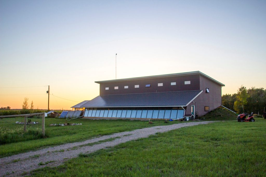
Figure 1: Passive Solar Home Near Elkhorn, Canada
Desirable amounts of low-energy-consumption heating and cooling are achieved, in the pictured home, by manually opening and closing blinds and windows to alter radiative and convective heat transfer into and out of the house. Although it reduces the amount of grid power used for heating and cooling, opening and closing the blinds and windows is repetitive and labour-intensive. This makes it an excellent candidate for automation.
Deciding when to and how much to open the blinds and windows is not trivial. A great deal of knowledge about thermal behaviour or experience about how the temperature in the home will change is needed to make the right decision. This decision-making process may be well addressed using machine learning—a data-driven method that removes the need for creating a definitive mathematical model of the system being controlled.
1.2 Literature Review
This discussion about simultaneously managing building energy consumption and internal environmental quality is paraphrased from Zhang et al. ‘s [1] discussion of the topic in their recent paper On the joint control of multiple building systems with reinforcement learning.
Reducing the trade-offs between performance and resource expenditure drives innovation in most industries, and building energy is not exempt. The contradiction between indoor environmental quality (IEQ) and energy savings is well-understood and has been the focus of many researchers over recent decades [1].
Indoor environmental quality encompasses many factors including temperature, humidity, light, and sound control. HVAC is an essential and non-trivial portion of indoor environment quality (IEQ) control problems because of the amount of energy it requires, the influence of user setpoints, thermal mass, and Spatio-temporal variability [1].
Energy consumption depends on the climate, but statistics show that heating and cooling systems account for a substantial amount of energy consumption on a national level. In commercial buildings, the subsystems with the largest energy consumption are HVAC and lighting [1]. In the UK, the estimated energy consumption for these two systems is 40% of all commercial building energy consumption [2]. And in Canada, where the climate is colder on average, that figure is 70% [3].
Innovators have addressed the IEQ-energy consumption contradiction in myriad ways. Applications of automation and control applications targeted at mitigating this trade-off can be classified as rule-based, model-based, and model-free methods [4] [1]:
- Rule-Based Methods – Rule-based control schemes are effectively a set of control rules defined by the intuition of an informed facility manager [4] [1]. Zhang et al. [1] say that the research shows that this type of control scheme can significantly reduce the amount of energy consumed by an HVAC system [5]. However, a significant drawback is a dependency on the quality of results on the quality of the control rules [1].
- Model-Based Methods – Model-based methods use physics- or data-driven models that effectively describe and predict the behaviour of the dynamic system [4]. Low-order heat-transfer functions have been used to control buildings with some success [6] [7]. Still, proper identification of the high-order heat-transfer functions that accurately characterize a real-world situation can be quite difficult [1]
- Model-Free Methods – Model-free methods bypass the need for intuition- or data-driven models by learning control policies through (trial and error) interactions with the systems they control [4]. Despite the broad application of reinforcement-learning (RL) models to building system control in recent years, their relative performance, stability, and convergence speed have not been well-studied [1].
Applicability of Machine Learning
The most recent automation and control approach with perhaps, the greatest potential has been machine learning. Howard and Gugger [8], in their 2020 publication Deep Learning for Coders with fastai & PyTorch, outline several inherent advantages and limitations of machine learning:
Table 1: Inherent Advantages and Disadvantages of Machine Learning
|
Advantages |
Disadvantages |
|
|
Zhang et al. [1] cite other researchers, saying that model-free or “machine learning” methods have been a recent approach to building system control [9]. Three reinforcement learning types are commonly used [1]:
- Q-learning (value-based) – Q-learning algorithms “update action values (i.e., Q-values) for each state based on the observation.” [1]
- Actuator Critic – Actuator critic algorithms “learn the control policy and the Q-values to update the control policy.” [1]
- Policy Gradient – Policy gradient algorithms “are… the least sample efficient, yet are more stable than other RL algorithms.” [1] Of the 77 studies reviewed in Reinforcement learning for building controls: The opportunities and challenges, Wang and Hong [9] found that 75% used value-based algorithms.
Previous Work
In On the Joint Control of Multiple Building Systems with Reinforcement Learning, Zhang et al. [1] demonstrate that with model-free methods, “11% and 31.8% more energy can be saved respectively in heating and cooling seasons over rule-based baselines that control the same [commercial] buildings.” Their [1] contributions regarding,
- state-of-the-art reinforcement learning control schemes,
- the contradictions between energy consumption, thermal comfort, visual comfort, and
- the performance of the proposed methods in joint control of energy systems when occupancy behaviour is known,
far exceed the scope of this study; however, the paper is recommended as further reading for building energy control, particularly for joint-control, commercial-building applications.
2. Scope & Objectives
The scope of this study is substantiated with a problem statement and clarified with an objective. Evaluation criteria provide quantifiable metrics for evaluation in later sections of this article.
2.1 Problem Statement
Opening and closing windows and blinds to make full use of the energy-saving design features in passive solar homes are repetitive, labour-intensive, and non-trivial. Automation via a machine-learning control application could make these actions more accessible and increase overall heating and cooling energy savings.
2.2 Objective
The objective of this article is to assess the usefulness of machine learning control applications in passive solar homes to
- control whether windows and blinds are open or closed, and
- minimize the amount of heating/cooling power used.
2.3 Evaluation Criteria
Conclusions of varying degrees of importance may be provided by this study.
For the control application studied in this article,
Feasibility is indicated by evidence of successful control of the windows and blinds in a passive solar house.
Novelty is indicated by evidence of successful control of the windows and blinds in a passive solar house, and energy savings greater than those achieved in similar recently published studies.
3. Methods & Procedure
The procedure for this study is typical for data science problems and follows the Drivetrain Approach put forward by Howard et al. [10]:
- An objective is defined.
- A set of actions to meet this objective is acknowledged.
- Data acquisition is considered and carried out.
- A model is built and evaluated.
The methods for this study are a unique subset of available resources, research capabilities, and project requirements. Among them are the following:
- EnergyPlus – A nodal building energy simulation engine.
- OpenStudio – A GUI used to increase control and convenience when using EnergyPlus.
- Google Sketchup – A CAD software used to define the geometry of the building being simulated in EnergyPlus
- Deep Learning for Coders with fastai and PyTorch: AI Applications without a PhD [8] – A book, with an accompanying course, written by Howard and Gugger.
- Google Colab – An JupyterNotebooks style API with remote GPUs to conveniently and quickly train neural networks.
- Python – A flexible modern coding language based on C.
- PyTorch – A Python library with unique functionality to process typical data types quickly on GPUs.
- fastai – A Python library stacked on top of PyTorch with convenient machine learning architectures and training functions.
The implementation of procedure and methods, carried out in subsequent subsections of this article, are summarized in the table below:
Table 2: Methods & Procedure
|
Subsection |
Procedure |
Methods |
| Parametric dependencies are recognized using engineering judgment, and data is collated by simulating the relevant circumstances. |
|
|
| A machine learning architecture is selected and qualitatively analyzed with a theoretical breakdown. |
|
|
| the architecture is implemented and trained to form a model which is quantitatively evaluated on its predictive power. |
|
3.1 Data: Building Energy Simulation
Two important areas of data acquisition are addressed here: First, what data is actually needed, under the heading Control System and Parametric Dependencies; and second, how that data is actually collated, under the heading EnergyPlus Building Energy Simulation.
Control System and Parametric Dependencies
Defining a control system simplifies the real-world scenario being studied while preserving all essential parametric dependencies. Parameters that are relevant and depend on one another will comprise the dataset used to train the control application.
Aspects such as thermal loads, an auxiliary solar water-heating system, internal geometry (e.g. furniture), and humidity are ignored. All heat transfer into and out of the building influences temperature regardless of whether by conduction, convection, or radiation. Convection is controlled by opening and closing windows. Radiation is controlled by opening or closing blinds. And, the HVAC makes up for changes toward the user’s setpoint that cannot be achieved otherwise. Each action, whether it be opening or closing windows or blinds or heating or cooling with the HVAC system, will affect the interior temperature of the home. Because of these dependencies, understanding what happens to all of these parameters when something inside the building is changed is critical:
Constraints
- Temperature Setpoint Array
Control (Independent) Parameters
- Window Open Array
- Blind Ope Array
Dependent Parameters
- Indoor Temperature
- Indoor Temperature Gradient
Invariable Parameters
- Outdoor Temperature
- Sun Angle Array
- Sun Intensity Array
Dependant Parameter to be Minimized
- Heating & Cooling Power Array
A block diagram representation of the control system can help visualize the role these parameters play on the system as a whole:
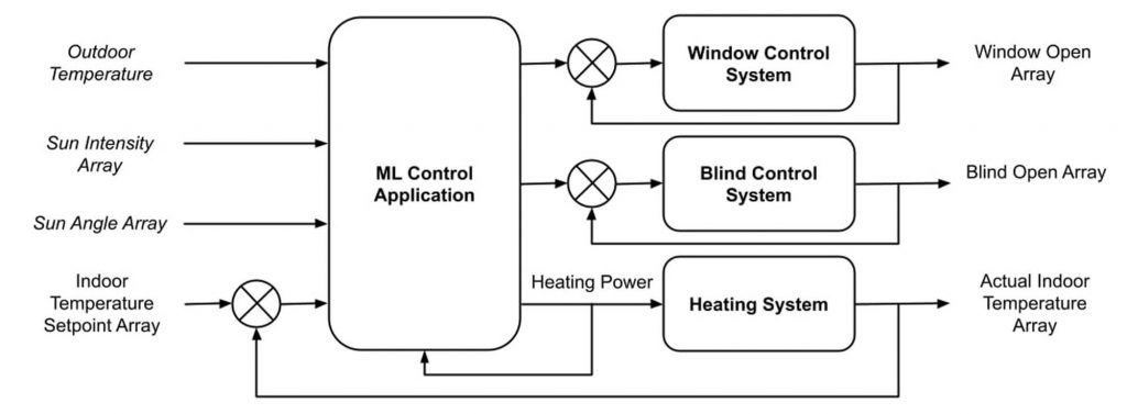
Figure 2: Passive Solar House Control System
The machine learning (ML) control application is given a set of inputs about the outdoor conditions and an error rate indicating the difference between desired and actual indoor conditions and is tasked with the objective outlined above. Its outputs are a set of commands for the amount to open or close windows and blinds as well as an amount of power sent to a heating system.
Each of the parameters identified as relevant and/or dependent in this subsection should be included in the collated dataset.
EnergyPlus Building Energy Simulation
Historically, both experimental apparatuses and computer-driven simulations have been used to validate scientific theses, particularly in the field of engineering.
Evins [11], a building-energy researcher and instructor at the University of Victoria, explained that data has been a stumbling block in the building-energy research field. Often, datasets are available, but not enough information about where they came from is available to make these sets useful for all applications. This is relevant because all machine learning is, by nature, heavily data-dependent. Moreover, in specific applications, like thermo- and fluid-dynamics, more data can be obtained from computer-driven simulations than from analogous experimental apparatus’ because of the absence of spatial sensor constraints. For these reasons, a computer-driven simulation model is used for this study. Evins [11] suggests using EnergyPlus, a nodal building-energy simulator for constructing a computer-driven thermal.
EnergyPlus has features that allow radiative heat transfer impacted by blinds to be simulated with a simple shoebox model. Convective heat transfer, impacted by airflow through windows and blinds is, however, more difficult to model and is excluded from this study for that reason.
The shoebox model used to derive collated data for this study is a heavily modified adaptation of a shoebox model provided by Evins [11], and Lari [12]. A more detailed description of the EnergyPlus simulation setup is available in Appendix A. A sample of the first five rows of collated data generated by the simulation, after minor alterations in Google Sheets and an import to Google Colab, is provided below.
Table 3: Passive Solar House Dataset (First Five Rows)
| time_min | dateAndTime_month | dateAndTime_day | dateAndTime_hour | dateAndTime_minute | outdoorTemperature_degC | indoorTemperature_degC | indoorTemperatureGrad_degCPerMin | indoorTemperatureSP_Heating_degC | indoorTemperatureSP_Cooling_degC | sunAngle_Azimuth_deg | sunAngle_Altitude_deg | sunAngle_Hour_deg | sunIntensity_Diffuse_WperSqm | sunIntensity_Direct_WPerSqM | districtHeating_J | districtCooling_J | surfaceShadingDeviceIsOnTimeFraction_SouthFacingWindow_bool | |
| 0 | 10 | 1 | 1 | 0 | 10 | 3.673583 | 14.068888 | -0.001559 | 15.6 | 26.7 | 3.767428 | -64.403334 | 181.76843 | 0.0 | 0.0 | 9.568201e+05 | 0.0 | 0 |
| 1 | 20 | 1 | 1 | 0 | 20 | 2.956917 | 14.053303 | -0.001559 | 15.6 | 26.7 | 1.559606 | -64.435170 | 179.26843 | 0.0 | 0.0 | 9.895696e+05 | 0.0 | 0 |
| 2 | 30 | 1 | 1 | 0 | 30 | 2.240250 | 14.036755 | -0.001655 | 15.6 | 26.7 | 6.871040 | -64.313708 | 176.76843 | 0.0 | 0.0 | 1.022900e+06 | 0.0 | 0 |
| 3 | 40 | 1 | 1 | 0 | 40 | 1.523583 | 14.039769 | 0.000301 | 15.6 | 26.7 | 12.114874 | -64.041185 | 174.26843 | 0.0 | 0.0 | 1.046125e+06 | 0.0 | 0 |
| 4 | 50 | 1 | 1 | 0 | 50 | 0.806917 | 14.024777 | -0.001499 | 15.6 | 26.7 | 17.243818 | -63.622467 | 171.76843 | 0.0 | 0.0 | 1.078738e+06 | 0.0 | 0 |
3.2 Architecture: Neural Networks & Collaborative Filtering
A neural network and collaborative filtering are used in conjunction in this study—the neural network to learn the data and make predictions, and collaborative filtering to handle the tabular data and pass it to the neural network as a matrix of activations.
Neural Networks
Neural networks are a topic of much research and development, and many forms are used in deep learning applications, including convolutional neural networks (CNNs) and recursive neural networks (RNNs). One of the most straightforward variations is used with collaborative filtering in this study. Its construction is similar to the neural network Howard and Gugger [8] built in Chapter 4 of their book.
A two-layer neural network can be written simply in the following way [8]:
w1 = init_params((28*28, 30))
b1 = init_params(30)
w2 = init_params((30, 1))
b2 = init_params(1)

def simple_net(xb):
    res = xb@w1 + b1
    res = res.max(tensor(0.0))
    res = res@w2 + b2
    return res
Looking at each of the constituent parts in turn,
- `w1` and `w2` are weight matrices,
- `b1` and `b2` are bias vectors, and
- `res.max(tensor(0.0))` constitutes a rectified linear unit (ReLU), which is a nonlinear function because it replaces all negative numbers with zero [8].
In `simple_net`,
- a vector, `xb`, (1 × 784) is multiplied by some weights, `w1`, (784 × 30) and summed with some biases, `b1`, (1 × 30) to produce `res` (1 × 30),
- `res` (1 × 30) is rectified by a non linear ReLU that turns all negative values into zero to produce a new `res` (1 × 30), and
- the new `res` (1 × 30) is multiplied by some weights, `w2`, (30 × 1) and summed with a bias, `b2`, (1 × 0) to produce the final `res` (1 × 0),
Non-linearity is essential in neural networks because superposition allows a series of linear multiplications and additions to be replaced with one single multiplication and addition [8]. This is not the case when non-linear functions are included. Each added set of linear and non-linear layers has a non-linear effect on the activations they form and can model more complex correlations between independent and dependent variables [8].
The universal approximation theorem says that “it can be mathematically proven that [the neural network presented above] can solve any computable function to an arbitrary level of accuracy [with the] right parameters for `w1` and `w2` and if [the] matrices are big enough!” [8]
The key to finding the right parameters for the weight matrices in a neural network is effectively using an error function, stochastic gradient descent (SGD), and some programming subtleties for implementation [8].
Written with methods from `PyTorch`’s `nn` class, this simple neural network can be simplified even further [8]:
simple_net = nn.sequential(
    nn.Linear(28*28, 30),
    nn.ReLU(),
    nn.Linear(30,1)
)
Howard and Gugger [8] developed a stochastic gradient descent (SGD) method to optimize the weight matrices in these neural networks for better predictions in Chapter 4 of their book:
def mnist_loss(predictions, targets):
    predictions = predictions.sigmoid()
    return torch.where(targets == 1, 1 - predictions, predictions).mean()

def calc_grad(xb, yb, model):
    preds = model(xb)
    loss = mnist_loss(preds, yb)
    loss.backward()

def train_epoch(model, lr, params):
    for xb, yb in dl:
        calc_grad(xb, yb, model)
        for p in params:
            p.data -= p.grad*lr
            p.grad.zero_()
There are several nuances of note in the above implementation:
- The `mnist_loss` function normalizes the `predictions`, then returns the `mean` of how far the `predictions` that should be zero are from zero and how far the `predictions` that should be one are from one [8].
- The `calc_grad` function calculates the gradient of the `mnist_loss` with the `.backward()` method [8]. It should be noted that in order to use the `PyTorch .backward()` method, `.requires_grad_()` has to have been assigned at each operation [8].
- The `train_epoch` function updates the parameters based on the gradient, `p.grad`, and learning rate, `lr`, without storing any information about the gradient by assigning the `.data` attribute, and then resets the gradient, `p.grad`, to zero [8].
Simplifications can be made by using of some of `PyTorch`’s library functions [8]:
calss BasicOptim:
    def __init__(self, params, lr):
        self.params
        self.lr = list(params)
        lr

    def step(self, *args, **kwargs):
        for p in self.params:
            p.data -=p.grad.data *self.lr

    def zero_grad(self, *args, **kwargs):
        for p in self.prarms:
            p.grad = None

opt = BasicOptim(linear_model.parameters(), lr)

def train_epoch(model):
    for xb, yb in dl:
        calc_grad(xb,yb, model)
        opt.step()
        opt.zero_grad()
When using the simplified `PyTorch` implementation, the following functionality is used:
- `linerar` functions are replaced with a `nn.Linear` object inherited from `PyTorch`’s `nn.Module` class [8]. The `nn.Linear` object declares and initializes a linear function with a matrix of weights and a vector of biases within a class structure [8].
In practice `fastai`’s `Learn.fit` method is used to train neural networks with stochastic gradient descent [8]:
learn = Learner(dls, nn.Linear(28*28, 1), opt_funct = SGD, loss_fucnt = mnist_loss, metrics= batch accuracy)

learn.fit(10, lr = lr)
Collaborative Filtering
Collaborative filtering is an architecture for handling tabular data that allows a neural network to learn correlations between items in a row or column [8]. Assume that the dataset is arranged as many rows, each abiding to some correlation between its columnated entries. If this is the case, a collaborative filtering model can learn the correlation that each row adheres to by
- assigning each row and column in the dataset an equal-length vector of random latent values,
- calculating predictions for a given entry by taking the dot product of that entry’s corresponding row and column latent value vector, and
- learning better latent values that produce more accurate predictions through stochastic gradient descent [8].
Collaborative filtering can be used to recommend movies to users without knowledge of genres, actors, directors, etc., by identifying trends in other users’ viewing history [8]. When generating a recommendation (or “prediction”) for a user, the model recognizes that movies not-yet-watched by that user but viewed by users with a similar viewing history would constitute a good recommendation [8]. In a more general sense, the model can learn correlations for which there might be a reason without knowing what that reason is [8].
The architecture used by `fastai.collab` is similar to the one developed and discussed by Howard and Gugger [8]:
class DotProduct(Module):
    def __init__(self, n_rows, n_cols, n_factors, y_range = (0, 5.5)):
        self.row_factors = create_params([n_row, n_factors])
        self.row_bias = create_params([n_rpws])
        self.col_factors = create_params([n_cols, n_factors])
        self.col_bias = create_params([n_rows])
        self.y_range = y_range

    def forward(self, x):
        rows = self.row_factors(x[:, 0])
        cols = self.col_factors(x[:, 1])
        res = (users * movies).sum(dim =1)
        res += self.row_bias[x[:, 0]] + self.col_bias[x[:, 1]]
        return sigmoid_range(res, *self*y_range)

model = DotProduct(n_rows, n_columns, 50)
learn = Learner(dls, model, loss_func = MSELossFlat())
The `DotProduct` class is designed to compute the prediction for a tabular entry by calculating the dot product of that entry’s associated row and columns latent value vectors while allowing reverse operations to be performed during training [8]. There are a few programming nuances included in the class definition above:
- Embedding is one way of improving efficiency and speed by using array lookups of one-hot-encoded matrix lookups [8].
- `Module` is inherited by `DotProduct` so that all of its functionality can be used [8].
- The argument `x` of `.forward()` is a matrix with two columns, the 0-th of which contains the indices for row’s (independent variables’) latent factors, and the 1-th of which contains the indices for the column’s (dependant variable) latent factors [8].
- `y_range` defines the range for regression, which is relevant when the dependent variable, for which predictions are made, is continuous [8].
- Biases between correlations are accounted for by adding latent values to the row’s (independent variables’) latent value vectors. The addition of too many latent values can result in overfitting [8].
- Regularization is used to simplify the model’s fit to the training data and reduce the chances of overfitting. It is done with weight decay, otherwise known as L2 linearization, which is the sum of all the weights squared to the loss function to avoid them growing too large [8].
- `PyTorch`’s `nn.Parameter()` and `nn.Linear()` methods are used to avoid the necessity of embeddings [8].
While the `DotProduct` class is suitable for learning latent value vectors with stochastic gradient descent, it must be adapted for use with a neural network [8]:
embs = get_emb_sz(dls)

class CollabNN(Module):
    def __init__(self, user_sz, item_sz, y_range = (0, 5.5), n_act = 100):
        self.user_factors = Embedding(*user_sz)
        self.item_factors = Embedding(*item_sz)
        self.layers = nn.Sequential(user_sz[1] + item_sz[1], n_act), nn.ReLU(), nn.Linear(n_act, 1))
        self.y_range = y_range

    def forward(self, x):
        embs = self.user_factors(x[:,0]), self.item_factors(x[:, 1])
        x = self.layers(torch.cat(embs, dim = 1))
        return sigmoid_range(x, *self.y_range)

model = CollabNN(*embs)
learn = Learner(dls, model, loss_func = MSELossFlat())
learn.fit_one_cycles(5, 5e-3, wd = 0.1)
The `CollabNN` class replaces learning latent value vectors using stochastic gradient descent with a neural network [8]. It includes the following nuances to actualize this:
- Embeddings are concatenated using `get_emb_sz` so that they can be passed to a neural network as a matrix of activations [8].
- `CollabNN` creates an embedding layer and uses `embs` sizes [8].
- `self.layers()` is a series of two linear and one non-linear layers that constitute a mini neural network [8].
- In `.forward()`, the embeddings are applied, the results are concatenated, and the activation matrix is passed to `self.layers()` [8].
- `sigmoid_range(x, lo, hi)` normalizes `x` to be between `lo` and `hi` by shifting and scaling the sigmoid function of `x` [8].
Other details exceed the scope of this article but are available in Chapter 8 of Howard and Gugger’s book [8].
fastai Implementation
For this study, `fastai.collab`’s predefined `tabular_learner` is used to create a collaborative filtering model with a two-layer neural network of 500 and 200 activations respectively [8]:
learn = tabular_learner(dls, y_range = (0, 1), layers = [500,250], n_out = 1, loss_func = F.mse_loss)
For `learn`, the following parameters are specified:
- `dls` is the `dataloaders` passed to the architecture [8]. (A `dataloaders` object is a packet of data from the dataset, structured to be handled by the `tabular_learner` in an efficient way [8].)
- `y_range` is the range for regression.
- `layers` specifies the number of layers in the neural network and the number of activations at each layer.
- `n_out` specifies the number of dependent variables.
`loss_func` specifies a method of calculating the loss used in stochastic gradient descent.
3.3 Modeling: Data Interpretation, Refinement, & Training
With an architecture defined, data interpretation, data refinement, and training must be discussed to cover the second portion of creating a model capable of achieving the defined objective.
Splitting Date and Time
The `dataloaders` class is passed a `TabularPanda` that specifies which portion of the dataset should be set aside for training [8].
The training and validation sets are often assigned randomly, but since the problem under investigation is a time series problem, a sequential split using Howard and Gugger’s method from Chapter 9 of their book [8] is made instead:
cond = (df.time_min < 420490)
train_idx = np.where( cond)[0]
valid_idx = np.where(~cond)[0]

splits = (list(train_idx), list(valid_idx))
Since the dataset contains 52,560 data points (one every 10 minutes over the course of the year), this split allocates the first 80% of data points to training and the subsequent 20% to validation.
Identifying and Removing Time-Dependant Data
As was discussed in §3.1, the rule used to create the dataset was closing the blinds between 12:00 pm and 4:00 pm during the summer months. To avoid the model learning these time rules instead of the correlation between blocking out sunlight to cool the building, all time data used as an independent parameter when making the dataset is removed. Included in this list are,
- `time_min`,
- `dateAndTime_month`,
- `dateAndTime_day`,
- `dateAndTime_hour`, and
- `dateAndTime_minute`.
This data is removed with the following code, following an example from Chapter 9 of Howard and Gugger’s book [8]:
to_drop = ['time_min',
           'dateAndTime_month',
           'dateAndTime_day',
           'dateAndTime_hour',
           'dateAndTime_minute']

xs_tindep = xs.drop(to_drop, axis=1)
valid_xs_tindep = valid_xs.drop(to_drop, axis=1)
Inferences about low-importance data, redundant data, and partial dependencies are made by interpreting what a random forest learns about the data. Random forests claim superiority over neural networks for analyzing data because they form a predictable structure with a known algorithm, while the parameters of a neural network often carry a more hidden meaning. Random forests are an extension of decision trees, based on Breiman’s work on Bagging Predictors [13], which use aggregated predictions from multiple decision trees constructed with random subsets of the data [8]. Implementation is not discussed here for brevity but can be found in Chapter 9 of Howard, and Gugger’s book [8].
Identifying and Removing Low-Importance Data
Data importance can be identified by parsing a decision tree and determining the error reduction associated with splits made based on each independent variable [8]:
def rf_feat_importance(m, df):
    return pd.DataFrame({'cols':df.columns, 'imp':m.feature_importances_}).sort_values('imp', ascending=False)

fi = rf_feat_importance(m, xs_tindep)
fi[:12]
This gives a table of feature importances similar to this:
Table 4: Feature Importances
|
index |
cols |
imp |
| 6 | sunAngle_Altitude_deg | 0.3138139529763225 |
| 5 | sunAngle_Azimuth_deg | 0.1647876165353201 |
| 8 | sunIntensity_Diffuse_WperSqm | 0.1437438455583515 |
| 0 | outdoorTemperature_degC | 0.10281190142470335 |
| 11 | districtCooling_J | 0.09900020363297138 |
| 7 | sunAngle_Hour_deg | 0.07179755129289568 |
| 1 | indoorTemperature_degC | 0.04073497721056296 |
| 9 | sunIntensity_Direct_WPerSqM | 0.03356974973425223 |
| 2 | indoorTemperatureGrad_degCPerMin | 0.021612175481768702 |
| 10 | districtHeating_J | 0.008100017210116954 |
| 4 | indoorTemperatureSP_Cooling_degC | 2.800894273454708e-05 |
| 3 | indoorTemperatureSP_Heating_degC | 0.0 |
For ease of interpretation, this information is plotted as a bar graph [8]:
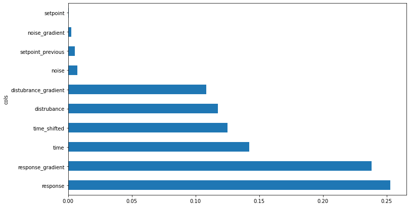
Figure 3: Feature Importance
Independent variables with the longest bars are the most important, while those with the shortest are the least important [8]. The least important ones can be removed by setting an importance threshold of 0.005 [8]. Independent variables with less importance will be removed. In this case,
- `indoorTemperatureSP_Heating_degC`,
- `indoorTemperatureSP_Heating_degC`, and
- `districtHeating_J`
are included in that list. When these parameters are removed, the validation root-mean-squared-error (RMSE) of the model goes from 0.0120 to 0.0062, indicating an increase in accuracy of the model’s predictions.
Identifying and Removing Redundant Data
Data redundancy is identified by recognizing which independent variables have similar importances [8]. For ease of interpretation, this information is plotted as a cluster graph [8]:
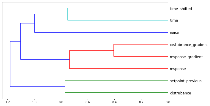
Figure 4: Feature Similarity
Independent variables that are joined closer to the right, represent those that are most similar, whereas those joined further to the left are the least similar [8]. In some cases, one of the independent variables in a similar pair might be redundant [8]. To check, a baseline out-of-bag score is calculated to be 0.9471, and other out of bag scores are calculated when each of the independent variables in the predominant similar data pairs is removed in turn:
Table 5: Feature Similarity OOB Score
| Similar Independent Variable Pairs | Independent Variables | Associated Out-of-Bag Score |
| Most-Similar Pair | sunIntensity_Diffuse_WperSqM | 0.9480 |
| sunAngle_Altitude_deg | 0.8946 | |
| Second-Most-Similar Pair | indoorTemperature_degC | 0.9456 |
| outdoorTemoerature_degC | 0.9435 |
The out-of-bag score (OOB) is a value returned by `sklearn`, where zero represents a completely random model, and one represents a perfect model [8]. The model gets better when `sunIntensity_Diffuse_WperSqM` is removed and only deteriorates marginally when `outdoorTemperature_degC` is removed, and when both are removed simultaneously, the out-of-bag score decreases marginally to `0.9445`. The `0.26%` loss in the model’s predictive power is worthwhile and both `sunIntensity_Diffuse_WperSqM` and `outdoorTemperature_degC` are removed.
Note that `outdoorTemperature_degC` is considered for removal before `indoorTemperature_degC`, even though the data suggests that the reverse should be considered. This is because the difference in model deterioration by removing either represents only a fraction of a percent difference and engineering judgment suggests that `indoorTemperature_degC` is more important to the model than `outdoorTemperature_degC`.
The dataset now has now been reduced to a simpler, yet nearly equally effective set of independent variables:
- `indoorTemperature_degC`
- `indoorTemperatureGrad_degCPerMin`
- `sunAngle_Azimuth_deg`
- `sunAngle_Altitude_deg`
- `sunAngle_Hour_deg`
- `sunIntensity_Direct_WPerSqM`
- `districtCooling_J`
- `surfaceShadingDeviceIsOnTimeFraction_SouthFacingWindow_bool`
Training the Neural Network
Having established a simple yet effective dataset, a neural network collaborative filtering architecture can be set up and trained using `fastai` library functions.
First, a few more steps are taken to implement the data modifications above and create a `dataloaders` for training:
df_nn = pd.read_csv(path/'20220315_Dataset_WindowShadingMLControlApp.csv', low_memory=False)

df_nn_final = df_nn[list(xs_final) + ['surfaceShadingDeviceIsOnTimeFraction_SouthFacingWindow_bool']]

cont_nn, cat_nn = cont_cat_split(df_nn_final, max_card=5, dep_var='surfaceShadingDeviceIsOnTimeFraction_SouthFacingWindow_bool')
df_nn_final[cat_nn].nunique()

df_nn_final = df_nn_final.astype({'surfaceShadingDeviceIsOnTimeFraction_SouthFacingWindow_bool': np.float16})

to_nn = TabularPandas(df_nn_final, procs_nn, cat_nn, cont_nn, splits=splits, y_names="surfaceShadingDeviceIsOnTimeFraction_SouthFacingWindow_bool")

dls = to_nn.dataloaders(1024)
This code block includes the following nuances.
- `df_nn` is a dataframe for the neural network collaborative filtering model, derived from the original dataset [8].
- The `df_nn_final` dataframe implements the data modifications made above by concatenating the `xs_final` list of independent variables and the dependent variable, `surfaceShadingDeviceIsOnTimeFraction_SouthFacingWindow_bool` [8].
- `cont_nn` and `cat_nn` are used to separate continuous and categorical variables in the dataframe by determining which have cardinalities less than five [8].
- Assigning the `.astype()` method to `df_nn_final` changes the type of the independent variable to a float, which is required for training [8].
- `to_nn` is the `TabularPanda` version of `df_nn_final` used by the data loader [8].
- Assigning `.dataloaders()` to `to_nn` creates a data loader, `to_nn`, which batches the data into mini batches of `1024` rows each for training [8].
Before training, the architecture is defined with an appropriate regression range for the dependant variable, `surfaceShadingDeviceIsOnTimeFraction_SouthFacingWindow_bool`:
y = to_nn.train.y
y.min(), y.max()

>>(0.0, 1.0)

learn = tabular_learner(dls, y_range = (0, 1), layers = [500,250], n_out = 1, loss_func = F.mse_loss)
In this code block, the following tools are used and parameters are defined:
- `y.min()` and `y.max()`, are used to determine the regression bounds of the independent variable [8].
- `dls` is the data loader created in the previous code block [8].
- `y_range = (0, 1)` defines the regression bounds for training [8].
- `layers = [500,250]` defines the number of activations in each of the layers of the neural network [8].
- `n_out = 1` defines the number of outputs for the model [8].
- `loss_func = F.mse_loss` defines the type of loss function used for stochastic gradient descent (SGD) [8].
This model is trained with `.fit_one_cycle()` for 50 epochs using learning rate, `lr`, selected with Smith’s [14] `.lr_find()` tool [8]:
learn.lr_find()

>>SuggestedLRs(valley=0.0030199517495930195)

learn.fit_one_cycle(50,1.2023e-3)
Training for 50 epochs yields a table of `train_loss` and `valid_loss` values similar to the one below:
Table 6: Training
| epoch | train_loss | valid_loss | time |
|
0 |
0.188047 | 0.090456 |
00:00 |
|
1 |
0.150686 | 0.050327 |
00:00 |
|
2 |
0.124051 | 0.040076 |
00:00 |
|
⋮ |
⋮ | ⋮ |
⋮ |
|
47 |
0.002654 | 0.000007 |
00:00 |
|
48 |
0.002517 | 0.000007 |
00:00 |
|
49 |
0.002484 | 0.000007 |
00:00 |
A continuous decrease in training loss, `train_loss`, and validation loss, `valid_loss`, indicates successful training through all 50 training epochs without the occurrence of overfitting. Typically, when overfitting occurs the training loss decreases as the model learns the data better, and the validation loss starts to increase as the model loses its interpolative and extrapolative power [8].
The root-mean-squared-error (RMSE) is calculated after 50 epochs of training:
preds, targs = learn.get_preds()
r_mse(preds,targs)

>>0.002632
4. Results & Discussion
Using the methods and procedure presented in the previous section, a machine learning control application that accurately predicts whether blinds should be open or closed was constructed and trained. This constitutes a demonstration of partial feasibility according to the definitions presented in §2.3.
In this section, the results are stated explicitly and substantiated by discussing why they may have occurred, including sources of accuracy and error. The results are measured against the objectives defined in §2.2, and recommendations for further work are made.
4.1 Results
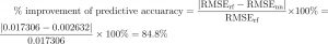
The model developed and trained in the previous section (§3) can predict whether blinds should be opened or closed with 99.7% accuracy:
![]()
This result represents an 85% improvement in accuracy over the random forest analog:
4.2 Discussion of Results
Such a high predictive accuracy is unusual from a deep learning model but is arguably expected in this case due to the simplicity of the dataset. The dataset was collated by running a simple shoebox building energy simulation with the control rule that blinds should be closed between 12:00 pm and 4:00 pm during the summer months (May–August), because these represent times when the sun would be most powerful and cooling by blocking the sun’s path into the home would be most noticed. Even though the independent variables used to create the rule (month and hour) were removed for training the control application, the correlation between independent variables and dependent variables is relatively simple. Moreover, the time-series split made to separate the validation set from the training set dictates that the validation set includes no instances when the blinds are to be closed.
4.3 Revisiting the Objective
The objectives of this study presented in §2.2 are revisited and used as a metric to measure the results. The objective of this study was to “assess the usefulness of machine learning control applications in passive solar homes to
- control whether windows and blinds are open or closed, and
- minimize the amount of heating/cooling power used.”
The neural network collaborative filtering control application developed can recommend whether blinds should be open or closed accurately; however, it cannot recommend whether windows should be open or closed to minimize the amount of grid power used for heating and cooling. Resources, experience, and time to support this functionality were not available when the procedure was developed and carried out.
The effect of opening and closing windows was excluded from the building energy simulation explained in §3.1 and Appendix A, because no dedicated method of doing so exists. While some researchers have adapted other functionality of EnergyPlus and Open Studio to accomplish similar results, doing the same fell outside the scope of this study.
Generating two simultaneous recommendations for two dependent parameters with a neural network collaborative filtering model while minimizing a third was not considered when developing the neural network collaborative filtering control application because similar examples were not included in this researcher’s broad and rapid review of the topic of machine learning.
Although no definitive methods are known to this researcher to add the functionality missing from the control application developed in this study, a few theoretical methods worth pursuing are listed and discussed briefly below, under “Recommendations for Future Work”.
4.4 Recommendations for Future Work
To develop a more useful conclusion, buoyancy-driven cooling—the cooling effect caused by opening and closing windows—should be simulated and included in the dataset. The control application should be modified to use this data to also recommend whether the windows should be open or closed. The Unmet Hours forum has discussed several methods to simulate this phenomenon for parametric studies in EnergyPlus and OpenStudio using measures. Other approaches can be found in building energy literature published on buoyancy-driven cooling, specifically.
Minimizing heating and cooling power must also be considered to develop a more useful conclusion. A few personable strategies to accomplish this are as follows:
- Iterative data optimization and model training – By doing this, the process of optimizing the control rules used to create the dataset is completely separated from training the model.
- Weighting the loss function by the normalized parameter to be optimized – By doing this, as the model learns to make more accurate predictions, in theory, it will also be learning to make more optimized predictions. Remember that the loss function represents the difference between the prediction generated and the actual value. It is minimized through training.
5. Conclusion
The feasibility of controlling blinds in a passive solar house with a machine learning control application can be concluded from the results of this study. The tested machine learning model could recommend whether blinds should be open or closed with a root-mean-squared error of 0.002632, based on the data, implying an accuracy of 99.7%.
This was done by
- collating a dataset with EnergyPlus—a building energy simulation engine,
- defining neural network collaborative filtering model of control of a passive solar homes blinds, and
- training the model with an appropriate learning rate and 50 epochs of training.
The objective of the study was to “assess the usefulness of machine learning control applications in passive solar homes to
- control whether windows and blinds are open or closed, and
- minimize the amount of heating/cooling power used.”
Successful control of windows and minimization of heating and cooling power could not be demonstrated.
Further work in the areas of
- modelling buoyancy-driven cooling through open windows in EnergyPlus and Open Studio,
- forming predictions for two dependent variables simultaneously with a neural-network collaborative filtering model, and
- Incorporating optimization in a neural network collaborative filtering recommender model,
must be done to form a more useful conclusion.
Acknowledgements
A few important contributors to this study are recognized in this section. These people provided endorsement and guidance at various stages of this project:
First, the supervisors of this project,
- Dr. Rustom Bhiladvala,
- Dr. Yang Shi,
are recognized for their endorsement of the topics studied.
The topic experts,
- Dr. Ralph Evins,
- Mr. Khosro Lari, and
- Mr. Liam Jowett-Lockwood,
are recognized for their consultation in the areas of building energy and machine learning.
And lastly,
- Mr. Joel Geico, and
- fastai Course Forums contributors
are recognized for providing detailed information about building energy and machine learning.
References
[1] T. Zhang, G. Baasch, O. Ardakanian, and R. Evins, “On the joint control of multiple building systems with reinforcement learning,” Proceedings of the Twelfth ACM International Conference on Future Energy Systems, 2021.
[2] U. S. Energy Information Administration, Energy Use Data Handbook. Available at https://www.eia.gov/outlooks/aeo/ (2021/12/27).
[3] N. R. Canada, Energy Use Data Handbook. Natural Resources Canada, 2019.
[4] X. Ding, W. Du, and A. Cerpa, “Octopus: Deep Reinforcement Learning for Holistic Smart Building Control,” in Proceedings of the 6th AMC International Conference for Energy-Efficient Buildings, Cities, and Transportation, AMC, 2019, pp. 326–335.
[5] O. Ardakanian, A. Bhattacharya, and D. Culler, “Non-intrusive occupancy monitoring for energy conservation in commercial buildings,” Elsevier: Energy and Buildings, vol. 179, pp. 311–323, 2018.
[6] S. Goyal, C. Liao, and P. Barooah, “Identification of multi-zone building thermal interaction model from data,” 2011.
[7] D. Zhou, Q. Hu, and C. Tomlin, “Quantitative comparison of data-driven and physics-based models for commercial building HVAC systems,” 2017.
[8] J. Howard and S. Gugger, Deep Learning for Coders with fastai & PyTorch: AI Applications Without a PhD, 1st ed. Sebastopol, CA: O’Reilly, 2020.
[9] Z. Wang and T. Hong, “Reinforcement learning for building controls: The opportunities and challenges,” Elsevier: Applied Energy, vol. 269, no. 115036, 2020.
[10] J. Howard, M. Zwemer, and M. Loukides, “Designing great data products,” www.oreilly.com, 28-Mar-2012. [Online]. Available: https://www.oreilly.com/radar/drivetrain-approach-data-products/. [Accessed: 29-Mar-2022].
[11] R. Evins, Professional Conversation, 2021.
[12] K. Lari, Professional Conversation, 2021.
[13] L. Breiman, “Bagging Predictors,” Technical Report No. 421, Sept 1994. [Online]. Available: https://www.stat.berkeley.edu/~breiman/bagging.pdf. [Accessed: 09 Apr 2022].
[14] L. N. Smith, “Cyclical Learning Rates for Training Neural Networks,” U.S. Naval Research Laboratory, Washington, DC, Technical Report, June 2015.
[15] B. L. S. LLC, “Table of contents: Input output reference – energyplus 9.6,” Big Ladder Software. [Online]. Available: https://bigladdersoftware.com/epx/docs/9-6/input-output-reference/. [Accessed: 09-Apr-2022].
Appendix A: Building Energy Simulation in EnergyPlus
An important component of the current study is a labelled dataset to train, validate, and test the final machine learning control system used to work towards greater energy savings. Since real, relevant datasets are difficult to obtain, a simulated dataset is generated using the nodal building energy simulation engine EnergyPlus. This appendix (A) explains the model built in EnergyPlus for which labelled data is obtained.
A.1 Introduction
An EnergyPlus shoebox model has been created to generate a dataset demonstrating the dependencies between relevant system parameters over a year. The final model used to obtain the training and validation datasets for this study is a version of a ShoeBox model provided by Evins [11] and Lari [12], altered to meet the current needs. It is the simplest representation of the situation under study—a low-energy-consumption residential home—that preserves all critical elements: solar radiation uptake, buoyancy-driven cooling, and baseboard heating.
Three pieces of software are used in conjunction to create this model:
- EnergyPlus – the nodal thermal simulation engine.
- Open Studio – a graphical user interface
- SketchUp – a computer-aided design (CAD) program used to define and alter the model’s geometry.
A.2 EnergyPlus & OpenStudio Model Definitions
The subsections below are organized to match the organization of EnergyPlus functionality in the OpenStudio GUI. For each subsection, there is a brief description as well as some screenshots explaining how that functionality was used.
Weather
Historical weather data for Victoria, British Columbia, is imported as “.epw” file, which defines the environmental conditions outside of the building for the study period [12].
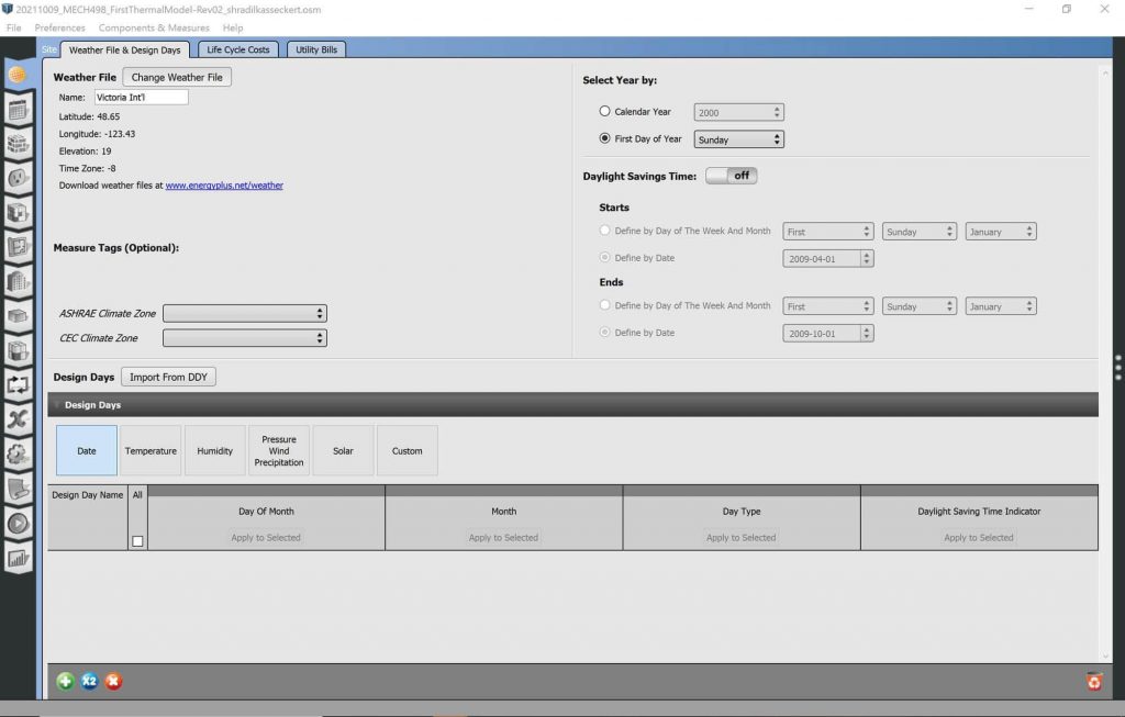
Image: EnergyPlus Weather
Schedules
Schedules are defined for occupancy, activity, lighting, electrical equipment, and infiltration. Each was imported as a boiler-plate schedule set for commercial office buildings modelled in EnergyPlus.
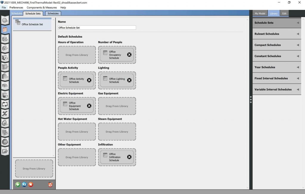
Image: EnergyPlus Schedules
Cooling and Heating Setpoint schedules were also predefined in the model supplied by Evins [11], and Lari [12].
A schedule to control a Venetian blind covering either window was developed specifically for this study, where blinds influence radiative heat flux entering the building. Either Venetian blind can be either open or closed. Accordingly, an on/off schedule type is used to control them. An effort is made to schedule the blinds to be open during the winter daylight hours and closed during what will likely be the hottest daylight hours of the summer. This schedule controls only the south-facing window, which is exposed to the most sun.
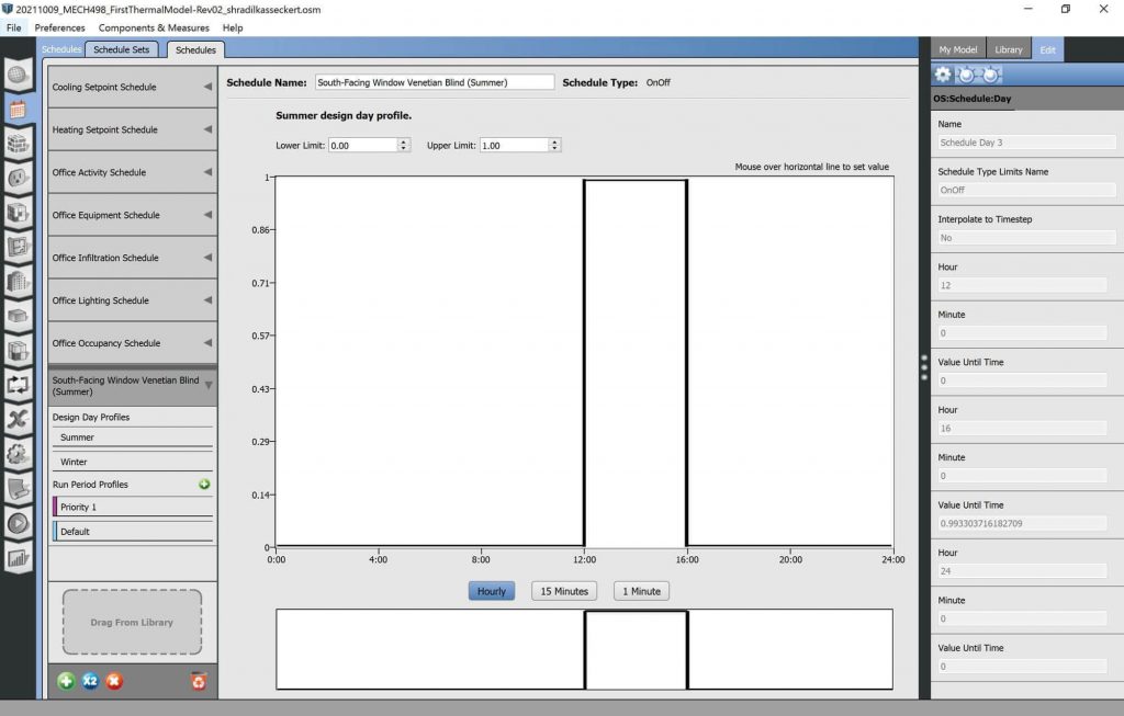
Image: EnergyPlus Schedules
Construction
Construction is relatively arbitrary for this study. It will impact absolute results but not relative ones between dependent variables. Knowing this, common constructions, predefined by Evins [11] and Lari [12], are left unaltered.
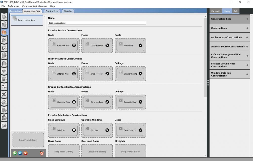
Image: EnergyPlus Construction
Loads
Loads may be defined for people, lights, internal mass, and various types of equipment. Again, for the sake of this study, these parameters have absolute and not relative effects and are left unaltered from Evins’ [11] and Lari’s [12] original model.

Image: EnergyPlus Loads
Space Types
Space types can be associated with a default construction set, default schedule set, design specification for outdoor air, space infiltration flow rate, and space infiltration effective leakage areas. Evins’ [11] and Lari’s [12] original model is left unaltered, which defined only one office space type with base construction, office schedule set, and office outdoor air.
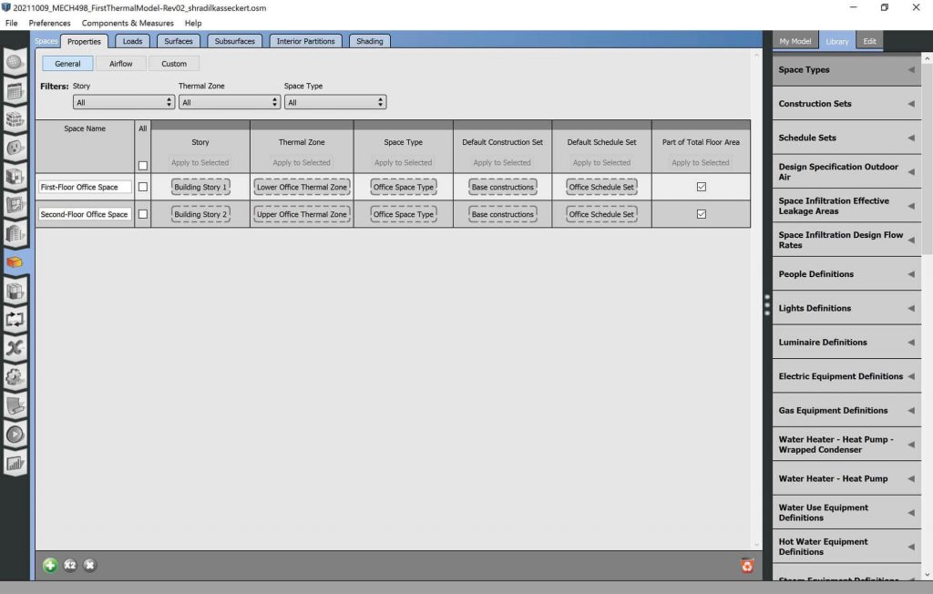
Image: EnergyPlus Space Types
Geometry
The geometry of a model is defined in the format of a “.idf” file [12]. Although the contents of these text files can be edited directly, it is often easiest to work on the geometry with the CAD software SketchUp [12].
The dimensions and orientation for the current shoebox model are two five-meter-long by five-meter-wide by three-meter-high (5m l × 5m w × 3m h) boxes stacked one on top of the other. Each has a four-meter-wide, by 1.5-meter-high (4m w × 1.5m h) window centred, one meter from the ground. The window for the lower box is in the south-facing wall, while the window for the upper box is in the north-facing wall. No floor/ceiling separates the lower box from the upper; however, they are defined as separate “thermal zones.”
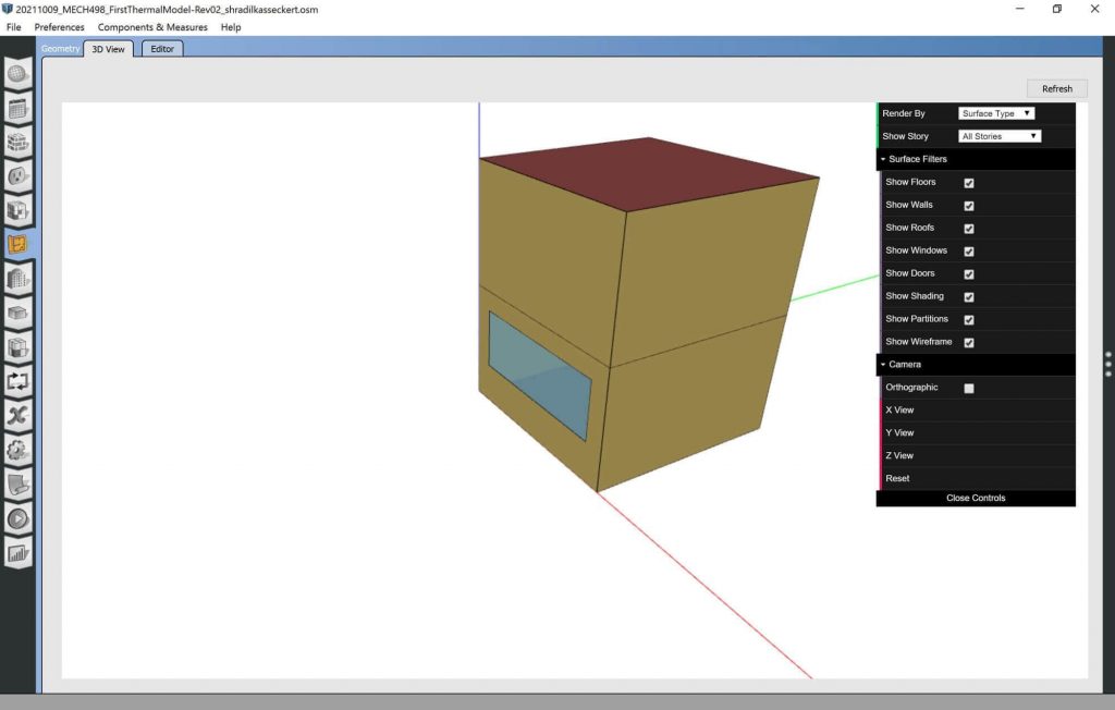
Image: EnergyPlus Geometry
Facility
The facility function of energy plus is not used for the purposes of this model.

Image: EnergyPlus Facility
Spaces
The spaces subsection of the OpenStudio EnergyPlus interface allows properties, loads, surfaces, subsurfaces, interior spaces, and shading to be assigned to different spaces. Two relevant specifications made for the two spaces in the current model are about the spaces themselves and the window subsurfaces.
The current model specifies the first and second stories as separate spaces, each with an associated thermal zone, but with the same space type, default construction type, and default schedule set.
The windows are defined as “OperableWindows,” indicating that they are opened and closed during the one-year simulation [12].
Likewise, the shading control type for the same windows is defined as “OnIfScheduleAllows,” indicating that a schedule will control the light transmission allowed by the associated Venetian blinds [12].
Loads remain unaltered from the original shoebox model provided by Evins [11] and Lari [12], and the interior partition functionality is not used.
Image: EnergyPlus Spaces
Thermal Zones
Two thermal zones are defined as stated in the ‘Geometry’ sub-section. This allows the temperature and temperature rate-of-change to be evaluated for both the hypothetical first and second floors.
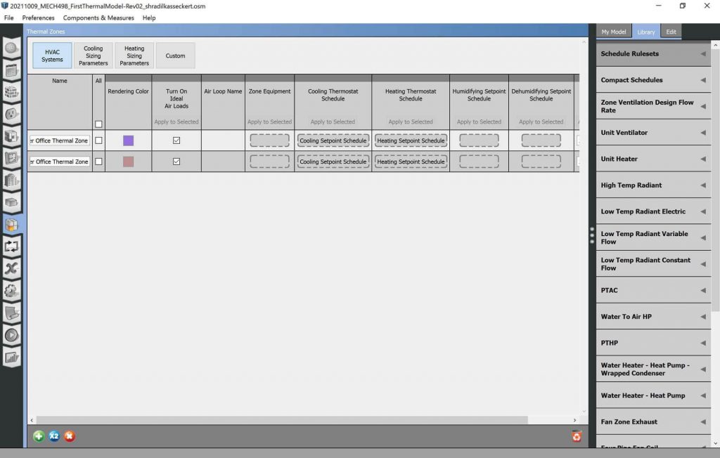
Image: EnergyPlus Thermal Zones
Output Variables
Using Big-Ladder Software’s [15] EnergyPlus Online Documentation, the outputs that correspond to the relevant parameters being observed has been selected and tabulated below:
Table: List of EnergyPlus/Open Studio Output Parameters
|
Parameter Type |
Parameter | EnergyPlus Output |
EnergyPlus Output Desc. |
| Constraint | Temperature Setpoint |
Zone Thermostat Heating Setpoint Temperature [C]
|
This is the current zone thermostat heating setpoint in degrees C. If there is no heating thermostat active, then the value will be 0. This value is set at each zone timestep. Using the averaged value for longer reporting frequencies (hourly, for example) may not be meaningful in some applications.
When the Thermostat:StagedDualSetpoint object is applied to the current zone, this output variable reports staged zone heating setpoint. When the staged number is not equal to zero, both staged heating and cooling setpoints are the same. When no cooling or heating is required, the staged heating setpoint is equal to the scheduled heating setpoint 0.5 * heating throttling range, and the staged cooling setpoint is equal to the scheduled cooling setpoint + 0.5 * cooling throttling range. |
|
Zone Thermostat Cooling Setpoint Temperature [C]
|
This is the current zone thermostat cooling setpoint in degrees C. If there is no cooling thermostat active, then the value will be 0. This value is set at each zone timestep. Using the averaged value for longer reporting frequencies (hourly, for example) may not be meaningful in some applications.
When the Thermostat:StagedDualSetpoint object is applied to the current zone, this output variable reports staged zone cooling setpoint. When the staged number is not equal to zero, both staged heating and cooling setpoints are the same. When no cooling or heating is required, the staged heating setpoint is equal to the scheduled heating setpoint 0.5 * heating throttling range, and the staged cooling setpoint is equal to the scheduled cooling setpoint + 0.5 * cooling throttling range. |
||
| Control (Independent) Parameter | Blind Open Array | Surface Shading Device Is On Time Fraction []
|
The fraction of time that a shading device is on an exterior window. For a particular simulation timestep, the value is 0.0 if the shading device is off (or there is no shading device) and the value is 1.0 if the shading device is on. (It is assumed that the shading device, if present, is either on or off for the entire timestep.) If the shading device is switchable glazing, a value of 0.0 means that the glazing is in the unswitched (light colored) state, and a value of 1.0 means that the glazing is in the switched (dark colored) state.
For a time interval longer than a timestep, this is the fraction of the time interval that the shading device is on. For example, take the case where the time interval is one hour and the timestep is 10 minutes. Then if the shading device is on for two timesteps in the hour and off for the other four timesteps, then the fraction of time that the shading device is on = 2/6 = 0.3333. |
| Dependant Parameter | Indoor Temperature | Zone Operative Temperature [C]
|
Zone Operative Temperature (OT) is the average of the Zone Mean Air Temperature (MAT) and Zone Mean Radiant Temperature (MRT), OT = 0.5*MAT + 0.5*MRT. This output variable is not affected by the type of thermostat controls in the zone, and does not include the direct effect of high temperature radiant systems. See also Zone Thermostat Operative Temperature. |
| Dependent Parameter | Indoor Temperature Gradient |
Calculated as a difference between discrete time steps:
|
|
| Invariable Parameter | Outdoor Temperature | Zone Outdoor Air Dry Bulb Temperature [C]
|
The outdoor air dry-bulb temperature calculated at the height above ground of the zone centroid. |
| Invariable Parameter | Sun angle | Site Solar Azimuthal Angle [deg]
|
The Solar Azimuth Angle (f) is measured from the North (clockwise) and is expressed in degrees. |
|
Site Solar Altitude Angle [deg]
|
The Solar Altitude Angle (b) is the angle of the sun above the horizontal (degrees). | ||
|
Site Solar Hour Angle [deg]
|
The Solar Hour Angle (H) gives the apparent solar time for the current time period (degrees). It is common astronomical practice to express the hour angle in hours, minutes and seconds of time rather than in degrees. You can convert the hour angle displayed from EnergyPlus to time by dividing by 15. (Note that 1 hour is equivalent to 15 degrees; 360° of the Earth’s rotation takes place every 24 hours.) | ||
| Invariable Parameter | Sun Intensity | Site Diffuse Solar Radiation Rate per Area [W/m2]
|
Diffuse solar is the amount of solar radiation in W/m^2 received from the sky (excluding the solar disk) on a horizontal surface. |
| Site Direct Solar Radiation Rate per Area [W/m2]
|
Site Direct Solar Radiation Rate per Area is the amount of solar radiation in W/m^2 received within a 5.7° field of view centered on the sun. This is also known as Beam Solar. | ||
| Parameter to be Minimized | Heating and Cooling Power | Zone Predicted Sensible Load to Setpoint Heat Transfer Rate [W]
|
This is the predicted sensible load in W required to meet the current zone thermostat setpoint. A positive value indicates a heating load, a negative value indicates a cooling load. This is calculated and reported from the Predict step in the Zone Predictor-Corrector module. For nearly all equipment types, the Predictor-Corrector evaluates the active heating and/or cooling setpoints, determines if the zone requires heating or cooling or is in the deadband, and then passes this single load to the equipment. This value is not multiplied by zone or group multipliers. |
| Plant Supply Side Heating Demand Rate [W]
|
This is the value of the net demand required to meet the heating setpoint of the loop. If the loop setpoint is met for the current HVAC timestep, Plant Supply Side Heating Demand Rate will equal the sum of the total heating demand from the demand side components on the loop. It will also equal the heating output of all heating equipment on the supply side of the loop plus any pump heat added to the fluid. For example, for a condenser loop with one ground loop heat exchanger and one pump serving one water-to-water heat pump, Plant Supply Side Heating Demand Rate will equal the ground loop heat transfer plus the pump heat to fluid, and it will also equal the heat pump condenser side heat transfer rate.
If the condenser loop setpoint is not met, Plant Supply Side Heating Demand Rate will equal the sum of the total heating demand from the demand side components on the loop plus the additional heating required to bring the loop flow to setpoint. If the loop remains off setpoint for successive timesteps, the demand required to return to setpoint will repeat in each timestep until the loop reaches setpoint. For this reason, Plant Supply Side Heating Demand Rate should not be summed over time, because it will overstate the demand whenever the loop is off setpoint. |
||
Each of these output variables can be added to the simulation in the “Output Variables” panel of OpenStudio or using the Add Output Variable measure.
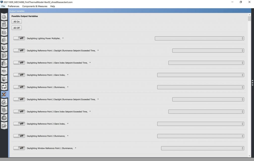
Image: EnergyPlus Output Variables
Simulation Settings
The relevant simulation settings are the date ranges and the number of time steps per hour. A whole year with six time-steps per hour is specified for this model, resulting in 52,560 data points in the final data set.
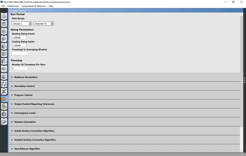
Image: EnergyPlus Simulation Settings
Measures
Measures allow parametric studies to be completed in EnergyPlus by changing parameters during a simulation period to mimic real-world applications [15]. No measures for parametric study are used for this simulation.
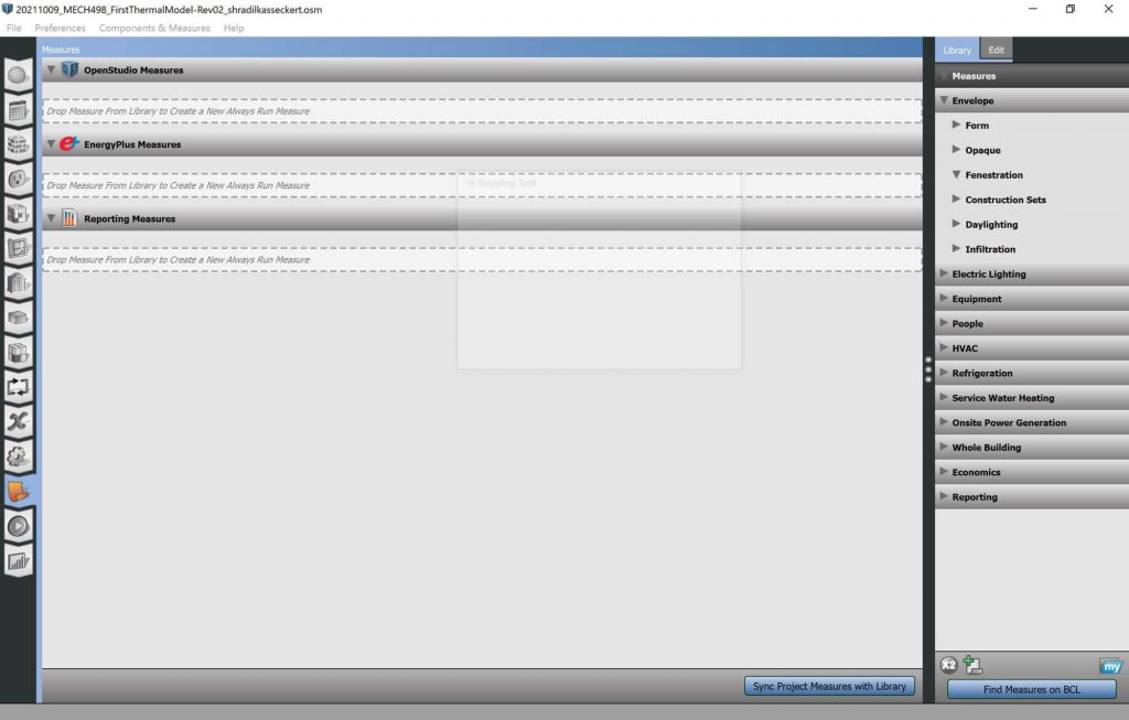
Image: EnergyPlus Measures
Appendix B: Google Colab Notebook
This appendix links the Google Colab Jupyter notebook used to execute all of the code used for this article’s Methods & Procedure section. Both the scripts and the outputs from the most recent compilation and execution can be seen by visiting this web address:
https://colab.research.google.com/drive/1aZXBQ_BJivNCFsLBAKnnmTawVJLhmfg_?usp=sharing
❗ This article was initially prepared as a report for MECH 498: Honours Thesis, supervised by Dr. Rustom Bhiladvala and Dr. Yang Shi, in partial fulfilment of the academic requirements of a mechanical engineering undergraduate degree at the University of Victoria.
Revision History:
|
Version |
Publication Date |
Description |
| V01, Rev.00 | 31 Dec. 2021 | Mid-Term Submission |
| V02, Rev.00 | 11 Apr. 2022 | Final Submission Draft |
| V03, Rev.00 | Final Submission* | |
* Pending revisions from supervisors Dr. Rustom Bhiladvala, and Dr. Yang Shi.